BiBiServ2 - RNAalishapes

RNAalishapes

Welcome

Submission

WebService

Download

Manual

References

Reset Session

RNAalishapes comes with the following different modes of predictions:

mfe

Computes the single energetically most stable secondary structure for the given RNA alignment. Co-optimal results will be suppressed, i.e. should different prediction have the same best energy value, just an arbitrary one out of them will be reported. This resembles the function of the program RNAalifold of the Vienna group (see [hof:fek:sta:2002] and [ber:hof:wil:gru:sta:2008]). If you only use mfe mode, consider switching to RNAalifold, because their implementation is much faster, due to sophisticated low level C optimizations.

subopt

Often, the biological relevant structure is hidden among suboptimal predictions. In subopt mode, you can also inspect all suboptimal solutions up to a given threshold (see parameters absolute deviation and relative deviation). Due to semantic ambiguity of the underlying "microstate" grammar, sometimes identical predictions will show up. As Vienna-Dot-Bracket strings they seem to be the same, but according to base dangling they differ and thus might even have slightly different energies. See [jan:schud:ste:gie:2011] for details.

shapes

Output of subopt mode is crowded by many very similar answers, which make it hard to focus to the "important" changes. The abstract shape concept [jan:gie:2010] groups similar answers together and reports only the best answer within such a group. Due to abstraction suboptimal analyses can be done more thorough, by ignoring boring differences (see option shape level).

probs

Structure probabilities are strictly correlated to their energy values. Grouped together into shape classes, their probabilities add up. Often a shape class with many members of worse energy becomes more probable than the shape containing the mfe structure but not much more members. See [vos:gie:reh:2006] for details on shape probabilities.

sample

Probabilistic sampling based on partition function. This mode combines stochastic sampling with a-posteriori shape abstraction. A sample from the structure space holds M structures together with their shapes, on which classification is performed. The probability of a shape can then be approximated by its frequency in the sample.

eval

Evaluates the free energy of an RNA molecule in fixed secondary structure, similar to RNAeval from the Vienna group.

Multiple answers stem from semantic ambiguity of the underlying grammar. It might happen, that your given structure is not a structure for the sequence. Maybe your settings are too restrictive, e.g. not allowing lonely base-pairs (lonely base pairs).

abstract

Abstracts a Vienna-Dot-Bracket representation of a secondary structure into a shape string.

outside

Applies the "outside"-algorithm to compute probabilities for all base pairs (i,j), based on the partition function [mcc:1990]. Output is a PostScript file, visualizing these probabilities as a "dot plot".

mea

Finds the secondary structure with the maximal sum of base-pair probabilities (MEA=maximal expected accuracy). The equivalent Vienna Package name is the 'centroid secondary structure', defined as 'The centroid structure is the structure with the minimum total base-pair distance to all structures in the thermodynamic ensemble.'.

In-/Output values

INPUT :: RNA sequence alignment

multiple RNA sequence alignment

INPUT :: RNA secondary structure

A Vienna dot-bracket formatted string, representing a seconday RNA structure.

OUTPUT :: output

Example output

The following image shows the output of the example call
RNAalishapes --mode probs --shape 5 --sci 1 --windowSi 50 --windowInc 14 --con mis --structureProbs 1 < tRNA.aln
Colored elements are not part of the output.

1		KSSUKYGURGYYYAGYu-GGY--ARRGCAYCWGSYUUUSRMSCWGAADKu	50
( -9.29 = -5.98 + -3.31)	0.8320257	.........(((.............))).(((((.......)))))....	(sci: 0.803)	0.9602453	[][]
( -7.38 = -5.14 + -2.24)	0.0375184	.............................(((((.......)))))....	(sci: 0.638)	0.0397234	[]
( -2.91 = -0.43 + -2.48)	0.0000266	.........((...))...((.....)).(((((.......)))))....	(sci: 0.252)	0.0000281	[][][]
( -1.50 = 1.38 + -2.88)	0.0000027	...((....(((.............)))..((((.......))))))...	(sci: 0.130)	0.0000032	[[][]]

15		GYu-GGY--ARRGCAYCWGSYUUUSRMSCWGAADKuCVBRGGUUCGARUC	64
( -7.38 = -5.14 + -2.24)	0.7722734	...............(((((.......)))))..................	(sci: 0.748)	0.8274852	[]
( -6.06 = -3.70 + -2.36)	0.0907037	.....((.....)).(((((.......)))))..................	(sci: 0.615)	0.1657448	[][]
( -3.91 = -1.48 + -2.43)	0.0027709	.....((.....)).(((((.......)))))........(((....)))	(sci: 0.397)	0.0066971	[][][]
( -1.59 = 0.89 + -2.48)	0.0000642	((...((.....)).(((((.......))))).........)).......	(sci: 0.161)	0.0000681	[[][]]
( 0.00 = 0.00 + 0.00)	0.0000049	..................................................	(sci: -0.000)	0.0000049	_

29		AYCWGSYUUUSRMSCWGAADKuCVBRGGUUCGARUCCYRKCGVDSSMR	76
(-15.60 = -10.79 + -4.81)	0.9238488	.(((((.......))))).....(((((.......)))))........	(sci: 1.168)	0.9999925	[][]
( -8.22 = -5.65 + -2.57)	0.0000058	.......................(((((.......)))))........	(sci: 0.615)	0.0000075	[]

Computation was done in window style, thus you see three different "result blocks", separated by newlines and sorted by "start position" Each result blocks has one "window info line" (green) and one or more "result lines" (blue). Lines are further divided into "fields", by two white space characters (red vertical lines). Contents of the fields are:

window info line
1. start position. Due to lengthy scores in result lines, start position has often leading white space characters.
2. "representative" for the (sub-)alignment that have been computed in this window. The representative can either be a "consensus" or a "most informative" sequence, depending on your choice of option consensus. In the example, we asked for most informative sequences.
3. "stop position"
result line
1. "score" of prediction, which is composed of an energy and a covariance part. Written as a Perl style RegEx, the format is
```
$$1\s=\s+$2\s\+\s+$3$
```
  , with $1 = combined score, $2 energy and $3 covariance. Should the start position consists of very many digits, it might happen that score has leading white space characters.
2. individual "structure probability" only if switched on via parameter structure probabilities
3. Vienna-Dot-Bracket representation of the secondary "structure".
4. structure conservation index ("sci") of the structure. This field only shows up, if structure conservation index is switched on. Format is:
```
$sci:\s+$1$
```
5. "shape probability" for the shape class, that is represented by the structure
6. "shape string" of the structure

Name

Description

mfe

Each result block contains only one result line, showing minimal free energy structure. Co-optimal results and shape probabilities are not computed for the sake of speed and thus not displayed.

subopt

Similar to mfe output, but each block can hold several result lines for sub-optimal structures. They are ascendingly sorted by their score.

shapes

Similar to subopt output, but structures with same shape strings are grouped. Result lines show the best member of a shape class (called "shrep"), which is determined by its score.

probs

Output as in the above example, result lines are descendingly sorted by shape probabilities

sample

Identical to probs output, since it computes the same information, but in a heuristic fashion.

Should you be interested in the concrete sampled structures, you can report them via option show samples. Output will have normal window info line, followed by the line

$1 samples, drawn by stochastic backtrace to estimate shape frequencies:

, where $1 is the value of numSamples. Traditional result lines begin after the line

Sampling results:

, which is surrounded by empty lines.

eval

Similar to mfe output, but should your grammar be semantically ambiguous (as "microstate" is) regarding Vienna-Dot-Bracket strings, you will get several result lines.

abstract

Output is just one line, holding the shape string for the given secondary structure.

outside

Outside mode produces a PostScript file, holding the probabilities of the base-pairs.
The "dot plot" shows a matrix of squares with area proportional to the base pair probabilities in the upper right half. For each pair (i,j) with probability above bppmThreshold there is a line of the form

i j sqrt(p) ubox

in the PostScript file, so that they can be easily extracted.

mea

Similar to mfe output. May contain several result lines due to co-optimal structures. The field "structure probability" here holds the sum of the MEA structures base-pairs, not the structure probability as in the other modes.

Parameter

Name

Description

Energy Deviation

relative deviation

relative deviation sets the energy range as percentage value of the minimum free energy. For example, when relative deviation is specified as 5.0, and the minimum free energy is -10.0 kcal/mol, the energy range is set to -9.5 to -10.0 kcal/mol.

relative deviation must be a positive floating point number; by default it is set to to 10 %.

It cannot be combined with absolute deviation.

absolute deviation

This sets the energy range as an absolute value of the minimum free energy. For example, when absolute deviation 10.0 kcal/mol is specified, and the minimum free energy is -10.0 kcal/mol, the energy range is set to 0.0 to -10.0 kcal/mol.

absolute deviation must be a positive floating point number. Cannot be combined with relative deviation.

Stochastic Options

number of samples

Sets the number of samples that are drawn to estimate shape probabilities.

In our experience, 1000 iterations are sufficient to achieve reasonable results for shapes with high probability. Thus, default is 1000.

show samples

You can inspect the samples drawn by stochastic backtrace if you activate show samples.

low probability filter

low probability filter sets a barrier for filtering out results with very low probabilities during calculation. The default value here is 0.000001, which gives a significant speedup compared to a disabled filter. Note that by turning on this filter, results are no longer guaranteed to be exact. This also influences shapes which have not been filtered out. For technical details, see [vos:gie:reh:2006]

Only floating point values between 0 and 1 are allowed, excluding 1.0, because otherwise virtually all results would be filtered out.

output probability filter

output probability filter sets a filter for omitting low probability results during output. It is just for reporting convenience. Unlike low probability filter, this option does not have any influence on runtime or probabilities beyond this value.

Only floating point values between 0 and 1 are allowed, excluding 1.0, because otherwise virtually all results would be filtered out.

decimals for probabilities

Sets the number of digits used for printing shape probabilities.

decimals for probabilities must be a positive integer number. The default value is 7.

structure probabilities

If activated, in addition to free energy also the probability of individual structures will be computed. To speed up computation, this calculation is switched off by default.

In MEA mode, the given probability is the sum of the base-pair probabilities used by the computed MEA structure and thus will likely be larger than 1.

Outside Options

bppmThreshold

Set the threshold for base pair probabilities included in the PostScript "dot plot" output.

Default is 0.00001.

Alignment Options

structure conservation index

The structure conservation index (SCI) is a measure for the likelihood that individual sequences will fold similar to the aligned sequences. It is computed as the aligned minimum free energy (MFE) divided by the average MFE of the unaligned sequences.

A SCI close to zero indicates that this structure is not a good consensus structure, whereas a set of perfectly conserved structures has SCI of 1. A SCI > 1 indicates a perfectly conserved secondary structure, which is, in addition, supported by compensatory and/or consistent mutations, which contribute a covariance score to the alignment MFE.

For further details see [was:hof:sta:2004].

For the sake of speed, SCI computation is switched off by default.

consensus

The input alignment will be represented in a single line. You can choose between

consensus: for a simple consensus sequence, determined by most frequent character. In case of co-optimals the alphabetically smaller base is reported.

mis the "most informative sequence": For each column of the alignment output the set of nucleotides with frequence greater than average in IUPAC notation.

Default is consensus.

pairing fraction

For a single RNA sequence it is easy to decide if positions i and j build a valid base pair. For alignments of RNA sequences this is more complicated, because some sequences might contain gaps. For exact definitions, see papers see [hof:fek:sta:2002] and [ber:hof:wil:gru:sta:2008] from the Vienna group.

Roughly speaking, the less pairingFraction, the more sequences must have a valid pair at positions i and j.

Default value is -200, meaning that at most half of the sequences must pair to let alignment positions i and j be a pair.

cfactor

Determines the relative strength of secondary structure energy vs covariance term. Default is 1.0.

nfactor

Determines how strongly pairs that cannot be formed by all sequences are penalised within the covariance term. Default value is 1.0.

Folding Options

grammar

How to treat dangling end energies for bases adjacent to helices in free ends and multi-loops.

nodangle: (-d 0 in Vienna package) ignores dangling energies altogether.

overdangle: (-d 2 in Vienna package) always dangles bases onto helices, even if they are part of neighbouring helices themselves. Seems to be wrong, but could perform surprisingly well.

microstate: (-d 1 in Vienna package) correct optimization of all dangling possibilities, unfortunately this results in an semantically ambiguous search space regarding Vienna-Dot-Bracket notations.

macrostate: (no correspondens in Vienna package) same as microstate, while staying unambiguous. Unfortunately, mfe computation violates Bellman's principle of optimality.

See [jan:schud:ste:gie:2011] for further details.

shape level

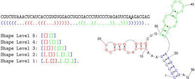
shape level is the level of abstraction or dissimilarity which defines a different shape. In general, helical regions are depicted by a pair of opening and closing brackets and unpaired regions are represented as a single underscore. The differences of the shape types are due to whether a structural element (bulge loop, internal loop, multiloop, hairpin loop, stacking region and external loop) contributes to the shape representation: Five types are implemented. Their differences are shown in the following example:

CGUCUUAAACUCAUCACCGUGUGGAGCUGCGACCCUUCCCUAGAUUCGAAGACGAG 
((((((...(((..(((...))))))...(((..((.....))..)))))))))..

Type	Description	Result
1	Most accurate - all loops and all unpaired	[_[_[]]_[_[]_]]_
2	Nesting pattern for all loop types and unpaired regions in external loop and multiloop	[[_[]][_[]_]]
3	Nesting pattern for all loop types but no unpaired regions	[[[]][[]]]
4	Helix nesting pattern in external loop and multiloop	[[][[]]]
5	Most abstract - helix nesting pattern and no unpaired regions	[[][]]

The following image also describes the differences between shape types:

temperature

The energy parameters used in the calculation have been measured at 37 C. Parameters at other temperatures can be extrapolated, but for temperatures far from 37 C results will be increasingly unreliable.

thermodynamic model parameters

Read energy parameters from a file, instead of using the default parameter set. See the RNAlib (Vienna RNA package) documentation for details on the file format.

Default are parameters released by the Turner group in 2004 (see [mat:dis:chil:schro:zuk:tur:2004] and [tur:mat:2010]). A visit of the aforementioned author's Nearest Neighbor Database might also be informative.

lonely base pairs

Lonely base pairs have no stabilising effect, because they cannot stack on another pair, but they heavily increase the size of the folding space. Thus, we normally forbid them. Should you want to allow them set lonely base pairs to 1.

lonely base pairs must be either 0 (=don't allow lonely base pairs) or 1 (= allow them).

Default is 0, i.e. no lonely base pairs.

ribosum scoring

Bases in two pairing alignment columns are not always identical. According to compensating mutations and the nature of the bases we score replacing one base with another differently. For example, replacing C by U might be more likely than C by A. These "distances" are expressed in form a distance matrix. By default, this matrix is a simple hamming distance matrix. A more advanced option is to use a "Ribosum" matrix, according to minimal and maximal pairwise sequence similarity.

The Vienna-Package states: "In addition ribosum scoring matrices are used. The matrix is chosen automatically according to the minimal and maximal pairwise identities of the sequences in the alignment file."

ribosum scoring must be either 0 (=hamming distance) or 1 (= ribosum distance).

Default is 0, i.e. hamming distance.

Input Style

window size

Instead of running the computation for the whole input sequence, you can apply a window style.

Imagine your input is a 4 mega bases genome, but you are looking for e.g. t-RNA, which is a small cloverleaf structure of say 80 bases. You don't want to have one prediction for the complete 4 MB genome, but predictions for 80 bases long parts of the genome.

If you input a positive window size, window style will be activated - as described above. After computation for the current window is done, it will be shifted by X bases to the right and computation for the next window starts. X can be modified via parameter window increment.

Overlapping parts are internally reused to save compute time.

window increment

Once you activate window style, by setting window size to a positive integer value, the sliding window will be shifted by X bases to the right after a window is computed. You can modify X with the parameter window increment.

Since there must be a overlap of at least one base between two windows, window increment must be smaller than window size. Only positive integer values are allowed.