BiBiServ2 - pKiss

pKiss

Welcome

Submission

WebService

Download

Manual

References

Reset Session

pKiss comes with the following different modes of predictions:

mfe

Computes the single energetically most stable secondary structure for the given RNA sequence. This structure might contain a pseudoknot of type H (simple canonical recursive pseudoknot) or type K (simple canonical recursive kissing hairpin), but need not to. Co-optimal results will be suppressed, i.e. should different prediction have the same best energy value, just an arbitrary one out of them will be reported.

subopt

Often, the biological relevant structure is hidden among suboptimal predictions. In subopt mode, you can also inspect all suboptimal solutions up to a given threshold (see parameters absolute deviation and relative deviation). Due to semantic ambiguity of the underlying "microstate" grammar, sometimes identical predictions will show up. As Vienna-Dot-Bracket strings they seem to be the same, but according to base dangling they differ and thus might even have slightly different energies. See [jan:schud:ste:gie:2011] for details.

enforce

Energetically best pseudoknots might be deeply burried under suboptimal solutions. Use enforce mode to enforce a structure prediction for each of the four classes: "nested structure" (as RNAfold would compute, i.e. without pseudoknots), "H-type pseudoknot", "K-type pseudoknot" and "H- and K-type pseudoknot". Useful if you want to compute the tendency of folding a pseudoknot or not, like in [the:ree:gie:2008].

local

Computes energetically best and suboptimal local pseudoknots. Local means, leading and trailing bases can be omitted and every prediction is a pseudoknot.

shapes

Output of subopt mode is crowded by many very similar answers, which make it hard to focus to the "important" changes. The abstract shape concept [jan:gie:2010] groups similar answers together and reports only the best answer within such a group. Due to abstraction suboptimal analyses can be done more thorough, by ignoring boring differences (see option shape level).

probs

Structure probabilities are strictly correlated to their energy values. Grouped together into shape classes, their probabilities add up. Often a shape class with many members of worse energy becomes more probable than the shape containing the mfe structure but not much more members. See [vos:gie:reh:2006] for details on shape probabilities.

cast

For a family of RNA sequences, this method independently enumerates the near-optimal abstract shape space, and predicts as the consensus an abstract shape common to all sequences. For each sequence, it delivers the thermodynamically best structure which has this common shape. Since the shape space is much smaller than the structure space, and identification of common shapes can be done in linear time (in the number of shapes considered), the method is essentially linear in the number of sequences. See [ree:gie:2005] for details. Should no common shape be reported, try to increase the amount of shape spaces being inspected via parameters relative deviation or absolute deviation.

eval

Evaluates the free energy of an RNA molecule in fixed secondary structure, similar to RNAeval from the Vienna group.

Multiple answers stem from semantic ambiguity of the underlying grammar. It might happen, that your given structure is not a structure for the sequence. Maybe your settings are too restrictive, e.g. not allowing lonely base-pairs (lonely base pairs).

If you input a (multiple) FASTA file, pKiss assumes that exactly first half of the contents of each entry is RNA sequence, second half is the according structure. Whitespaces are ignored.

abstract

Abstracts a Vienna-Dot-Bracket representation of a secondary structure into a shape string.

In-/Output values

INPUT :: RNA secondary structure

A Vienna dot-bracket formatted string, representing a seconday RNA structure.

INPUT :: RNA sequence(s)

A (multiple) FASTA file, containing RNA primary sequences.

INPUT :: RNA sequence

Exactly one RNA primary sequence.

INPUT :: RNA family

A family of at least two potentially related RNA sequences. This is not an alignment, since sequences can have different lengths.

OUTPUT :: output

Example output

The following image shows the output of the example call
pKiss --mode=probs --windowS 50 --windowInc 10 --outputLo 0.001 < test.mfa
Colored elements are not part of the output.

>example sequence
1	UGGCCGGCAUGGUCCCAGCCUCCUCGCUGGCGCCGGCUGGGCAACAUUCC	50
-25.20	..[[[[[[.....{{{{{{{.....]]]]]]...}}}}}}}.........	0.9903744	[{]}
-22.30	.[[[[[[[.{{...(((((......))))).]]]]]]]...}}.......	0.0067274	[{()]}
-21.10	..[[[[[[.{{...(((((......))))).]]]]]]..<<...}}..>>	0.0021679	[{()]<}>

11	GGUCCCAGCCUCCUCGCUGGCGCCGGCUGGGCAACAUUCCGAGGGGACCG	60
-24.00	....[[[[.{{{{{{{]]]].(((.....))).......}}}}}}}....	0.9364161	[{]()}
-21.40	...[[[[[[[.{{{{{........]]]]]]]........}}}}}......	0.0382784	[{]}
-20.00	[[.{{{{{{{.]]....<<.....}}}}}}}...>>.(((....)))...	0.0095886	[{]<}>()
-19.20	[[.{{{{{{{.]]....<<<....}}}}}}}.......>>>.........	0.0069825	[{]<}>
-19.80	[[.{{{{{{{.]].....<<....}}}}}}}.......((....)).>>.	0.0055529	[{]<}()>

>second example sequence
1	UGGCCGGCAUGGUCCCAGCCUCCUCGCUGGCGCCGGCUGGGCAACAUUCC	50
-25.20	..[[[[[[.....{{{{{{{.....]]]]]]...}}}}}}}.........	0.9903744	[{]}
-22.30	.[[[[[[[.{{...(((((......))))).]]]]]]]...}}.......	0.0067274	[{()]}
-21.10	..[[[[[[.{{...(((((......))))).]]]]]]..<<...}}..>>	0.0021679	[{()]<}>

11	GGUCCCAGCCUCCUCGCUGGCGCCGGCUGGGCAACAUUCCGAGGGGACCG	60
-24.00	....[[[[.{{{{{{{]]]].(((.....))).......}}}}}}}....	0.9364161	[{]()}
-21.40	...[[[[[[[.{{{{{........]]]]]]]........}}}}}......	0.0382784	[{]}
-20.00	[[.{{{{{{{.]]....<<.....}}}}}}}...>>.(((....)))...	0.0095886	[{]<}>()
-19.20	[[.{{{{{{{.]]....<<<....}}}}}}}.......>>>.........	0.0069825	[{]<}>
-19.80	[[.{{{{{{{.]].....<<....}}}}}}}.......((....)).>>.	0.0055529	[{]<}()>

You get two "answers" for the two input sequences, contained in "test.mfa". Each answer starts with an "identification line" (orange). Computation was done in window style, thus you see two different "result blocks" for each sequence, separated by newlines and sorted by "start position". (If input sequences have different lengths, output has different number of result blocks for the sequences). Each result blocks has one "window info line" (green) and one or more "result lines" (blue). Lines are further divided into "fields", by two white space characters (red vertical lines). Contents of the fields are:

identification line
1. sequence name: first character is the FASTA typical >, followed by the name of the sequence.
window info line
1. start position. Due to lengthy scores in result lines, start position has often leading white space characters.
2. "representative" is the sub-sequence that has been computed in this result block
3. "stop position"
result line
1. "free energy" in kcal/mol
2. Vienna-Dot-Bracket representation of the secondary "structure".
3. "shape probability" for the shape class, that is represented by the structure
4. "shape string" of the structure

Name

Description

mfe

Each result block contains only one result line, showing minimal free energy structure. Co-optimal results and shape probabilities are not computed for the sake of speed and thus not displayed. Also the shape string is not reported.

subopt

Similar to mfe output, but each block can hold several result lines for sub-optimal structures. They are ascendingly sorted by their free energy.

enforce

Compared to mfe output, result lines now contain a third field, which gives the class of the structure prediction. The four available classes have the hard coded ordering:

best 'nested structure',
best 'H-type pseudoknot',
best 'K-type pseudoknot' and
best 'H- and K-type pseudoknot'.

One energetically best result is returned for each class. For shorter sequences it might happen that a class contains no structures at all. For such a case the Vienna-Dot-Bracket field shows the string no structure available and the free energy field will be empty.

local

In local mode, results are for arbitrary sub-sequences of the input. Thus, start- and end- position become very important, but it gets complicated if you operate in window style, because you than have two levels of positions. First the window and second the local position within this window. That's the reason for a further "window position line":

=== window: x to y: ===

, where x and y are the start- and end- position of the current window. To retain the connection between positions and processed sub-string of the input sequence, the former window info line has now the fields 1) local start position, 2) processed sub-string and 3) local end position.

Output is sorted by two criteria: 1) window start position 2) free energy of local position. In case of energetically co-optimal results, they are further sorted by local start- and end- positions.

shapes

Similar to subopt output, enriched with shape strings, but structures with same shape strings are grouped. Result lines show the best member of a shape class (called "shrep"), which is determined by its free energy.

probs

Output as in the above example, result lines are descendingly sorted by shape probabilities

cast

Output of cast has its very own format, because your input is a family of related RNA sequences and result is common shapes for all family members. Here is an example output for the call
pKiss --mode=cast --abs 4.5 < test.mfa

Shape: ()

Score: -35.00

Ratio of MFE: 0.86

>seq1
1	CACACAAAGGCAGCGGAACCCCCCUCCUGGUAACAGGAGCCU	42
-10.00	.......................((((((....))))))...	R: 4	()
>seq2
1	AGGCAGCGGAAAUCCCCACCUGGUAACAGGUGCCUCUGC	39
-15.20	..((((.((.......((((((....)))))))).))))	R: 1	()
>seq3
1	CCUUUGCAGGCAGCGGAAUCCCCCACCUGGUGACAGGUGCCU	42
-9.80	.......................((((((....))))))...	R: 13	()

Shape: (()())

Score: -30.30

Ratio of MFE: 0.74

>seq1
1	CACACAAAGGCAGCGGAACCCCCCUCCUGGUAACAGGAGCCU	42
-9.60	.......((((...((....))..(((((....)))))))))	R: 6	(()())
>seq2
1	AGGCAGCGGAAAUCCCCACCUGGUAACAGGUGCCUCUGC	39
-11.70	..((((.((....)).((((((....))))))...))))	R: 3	(()())
>seq3
1	CCUUUGCAGGCAGCGGAAUCCCCCACCUGGUGACAGGUGCCU	42
-9.00	.......(((((..((......)).((((....)))))))))	R: 16	(()())

The RNA family might have several common shapes (two in the example), which are sorted by their combined free energy, called "Score". For each common shape the following lines are printed:

"common shape line", with fields:
1. Rank of common shape
2. common shape string
3. the Score of the common shape, which is the sum of free energies of the family member sequences.
4. Ratio of MFE, which is the Score divided by the sum of all minimal free energies of all family members, indendent of their shape class, i.e. if freely folded.
one identification line per family member
one window info line per family member
one result line per family member, where third field is the Rank of the shape class in shape mode

eval

Similar to mfe output, enriched with shape strings, but should your grammar be semantically ambiguous (as "microstate" is) regarding Vienna-Dot-Bracket strings, you will get several result lines. Please note that window style input would be nonsense, thus you get only one result block.

abstract

Output is just one line, holding the shape string for the given secondary structure. Again, window style input is nonsense

Parameter

Name

Description

Energy Deviation

relative deviation

relative deviation sets the energy range as percentage value of the minimum free energy. For example, when relative deviation is specified as 5.0, and the minimum free energy is -10.0 kcal/mol, the energy range is set to -9.5 to -10.0 kcal/mol.

relative deviation must be a positive floating point number; by default it is set to to 10 %.

It cannot be combined with absolute deviation.

absolute deviation

This sets the energy range as an absolute value of the minimum free energy. For example, when absolute deviation 10.0 kcal/mol is specified, and the minimum free energy is -10.0 kcal/mol, the energy range is set to 0.0 to -10.0 kcal/mol.

absolute deviation must be a positive floating point number. Cannot be combined with relative deviation.

Stochastic Options

low probability filter

low probability filter sets a barrier for filtering out results with very low probabilities during calculation. The default value here is 0.000001, which gives a significant speedup compared to a disabled filter. Note that by turning on this filter, results are no longer guaranteed to be exact. This also influences shapes which have not been filtered out. For technical details, see [vos:gie:reh:2006]

Only floating point values between 0 and 1 are allowed, excluding 1.0, because otherwise virtually all results would be filtered out.

output probability filter

output probability filter sets a filter for omitting low probability results during output. It is just for reporting convenience. Unlike low probability filter, this option does not have any influence on runtime or probabilities beyond this value.

Only floating point values between 0 and 1 are allowed, excluding 1.0, because otherwise virtually all results would be filtered out.

decimals for probabilities

Sets the number of digits used for printing shape probabilities.

decimals for probabilities must be a positive integer number. The default value is 7.

Pseudoknot Options

strategy

Strategy pKiss A: fast but sloppy

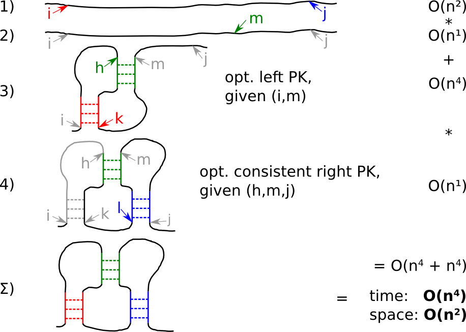
Strategy A makes the optimistic assumption that an optimal pseudoknot for the first half of the input sequence can be taken over to the kissing hairpin. The missing stem is adopted by an optimal, consistent pseudoknot for the second half:

for the given input, check all start- i and stop- j positions for a kissing hairpin
split the subword into two parts at m
find the optimal pseudoknot for the first part i to m, thus yielding indices h and k
find an optimal, consistent pseudoknot for the second part, i.e. determine l
do it vice versa and pick the energetically better solution

Strategy pKiss B: buying thoroughness by memory

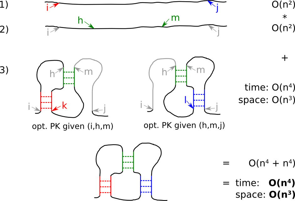
The overlay of two optimal pseudoknots must not necessarily yield an optimal kissing hairpin, since the overlay idea violates Bellman's principle of optimality. Thus the combination of two suboptimal pseudoknots might result in an energetically better kissing hairpin. This knowledge is the basis for Strategy B. This modification leads to higher memory consumption to store certain suboptimal pseudoknots.

for the given input, check all start- i and stop- j positions for a kissing hairpin
check for all positions h and m ...
... the overlay of a suboptimal pseudoknot (i,h,m) and a second suboptimal pseudoknot (h,m,j)

Strategy pKiss C: slow, low memory, but thorough

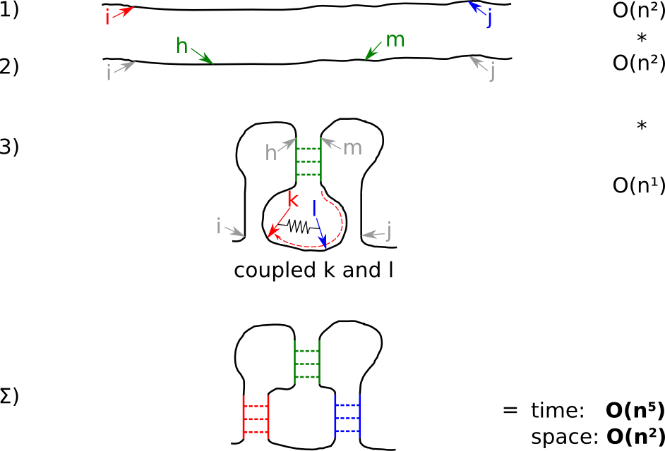
Since larger memory is often a harder problem than longer runtime, we alter Strategy B to trade memory for runtime. Strategy C avoids the extra storage required by Strategy B by re-computing the necessary information on demand. Coupling k and l reduces the runtime by one dimension.

for the given input, check all start- i and stop- j positions for a kissing hairpin
check for all positions h and m ...
... the energetically best kissing hairpin by iterating k and l in a coupled fashion.

Strategy pKiss D: very slow, but thorough

Strategy D is mainly for debugging. It is the direct application of the canonicalization rules known from pknotsRG, thus it has a very slow runtime of O(n⁶). Compared to strategies A to C and regarding the canonization concept, Strategy D is the only non-heuristic one. Thus, it returns the best results, but its runtime is often unaffordable.

for the given input, check all start- i and stop- j positions for a kissing hairpin
check for all positions h and m ...
and all positions k and l the energetically best kissing hairpin

Strategy pknotsRG

Strategy pknotsRG is the computation of canonical simple recursive pseudoknots as known from the program pknotsRG. It is the same as the first three steps from Strategy A. Choose this strategy if you want to completely turn off kissing hairpins.

Htype penalty

Thermodynamic energy parameters for pseudoknots have not been measured in a wet lab, yet. We can only guess reasonable values. Thus, you might want to set the penalty for opening a H-type pseudoknot yourself, via this parameter.

Htype penalty must be a floating point number. Default is 9 kcal/mol.

Ktype penalty

Ktype penalty must be a floating point number. Default is 12 kcal/mol.

maximal pseudoknot size

To speed up computation, you can limit the number of bases involved in a pseudoknot (and all it's loop regions) by defining a value for maximal pseudoknot size.

Only positive numbers are allowed. By default, there is no limitation, i.e. maximal pseudoknot size is set to input length.

minimal hairpin length

The canonical computation of pseudoknots requires a set of non-interrupted stems; two in the case of pknotsRG and three for kissing hairpins. These stems are pre-computed in O(n^2) time and space. A minimal size requirement, i.e. number of stacked base-pairs, for the stems constrains the number of results for the pre-computation and thus has a high impact on the overall runtime. With growing minimal size, more and more potential pseudoknots are ruled out and the results become less accurate.

For kissing hairpins, this does not affect the stem of the kiss for sterical reasons, but both stems of the hairpins.

Folding Options

shape level

Shape level is the level of abstraction or dissimilarity which defines a different shape. In general, helical regions are depicted by a pair of opening and closing brackets and unpaired regions are represented as a single underscore. The differences of the shape types are due to whether a structural element (bulge loop, internal loop, multiloop, hairpin loop, stacking region and external loop) contributes to the shape representation: Five types are implemented. Their differences are shown in the following example:

CGUCUUAAACUCAUCACCGUGUGGAGCUGCGACCCUUCCCUAGAUUCGAAGACGAG 
((((((...(((..(((...))))))...(((..((.....))..)))))))))..

Type	Description	Result
1	Most accurate - all loops and all unpaired	(_(_())_(_()_))_
2	Nesting pattern for all loop types and unpaired regions in external loop and multiloop	((_())(_()_))
3	Nesting pattern for all loop types but no unpaired regions	((())(()))
4	Helix nesting pattern in external loop and multiloop	(()(()))
5	Most abstract - helix nesting pattern and no unpaired regions	(()())

The following image also describes the differences between shape types:

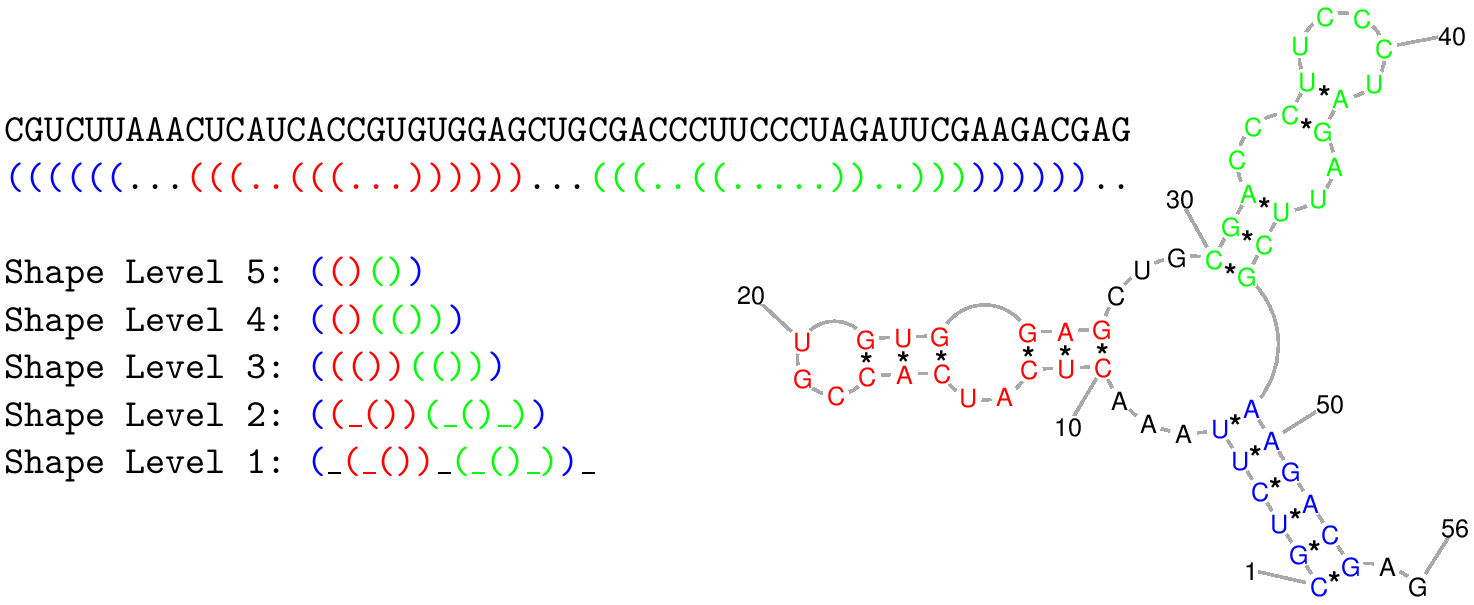
Please note that we use a slightly different definition of shapes, compared to the original RNAshapes program. Instead of square brackets we use parentheses, to keep the square brackets for pseudoknots. The level five shape for

AAGGGCGUCGUCGCCCCGAGUCGUAGCAGUUGACUACUGUUAUGU
..[[[[[..{{]]]]].....<<<<<<<<<..}}.>>>>>>>>>.

is for example

[{]<}>

temperature

The energy parameters used in the calculation have been measured at 37 C. Parameters at other temperatures can be extrapolated, but for temperatures far from 37 C results will be increasingly unreliable.

thermodynamic model parameters

Read energy parameters from a file, instead of using the default parameter set. See the RNAlib (Vienna RNA package) documentation for details on the file format.

Default are parameters released by the Turner group in 2004 (see [mat:dis:chil:schro:zuk:tur:2004] and [tur:mat:2010]). A visit of the aforementioned author's Nearest Neighbor Database might also be informative.

lonely base pairs

Lonely base pairs have no stabilising effect, because they cannot stack on another pair, but they heavily increase the size of the folding space. Thus, we normally forbid them. Should you want to allow them set lonely base pairs to 1.

lonely base pairs must be either 0 (=don't allow lonely base pairs) or 1 (= allow them).

Default is 0, i.e. no lonely base pairs.

Input Style

window size

Instead of running the computation for the whole input sequence, you can apply a window style.

Imagine your input is a 4 mega bases genome, but you are looking for e.g. t-RNA, which is a small cloverleaf structure of say 80 bases. You don't want to have one prediction for the complete 4 MB genome, but predictions for 80 bases long parts of the genome.

If you input a positive window size, window style will be activated - as described above. After computation for the current window is done, it will be shifted by X bases to the right and computation for the next window starts. X can be modified via parameter window increment.

Overlapping parts are internally reused to save compute time.

window increment

Once you activate window style, by setting window size to a positive integer value, the sliding window will be shifted by X bases to the right after a window is computed. You can modify X with the parameter window increment.

Since there must be a overlap of at least one base between two windows, window increment must be smaller than window size. Only positive integer values are allowed.