Startup possibilities
UniMoG can be started in console modus or with a graphical
user interface.
For using the console modus two parameters have to be
provided:
- The scenario: 1 = DCJ, 2 = rDCJ, 3 = HP, 4 = Inversion, 5 =
Translocatin, 6 = All scenarios at once
- The path to a single file containing all genomes which
should be analyzed
Example: java -jar UniMoG 5 path\to\genomefile.txt
path\to\genomefile2.txt
If no correct parameters are povided, UniMoG starts with the
graphical user interface.
Genome Representation
The loaded files have to contain at least two, but can contain
several genomes.
Every genome starts with a > followed by the genome
name.
In the following line(s) come the genes. 'Newlines' are
ignored.
Each chromosome is concluded by a closing parenthesis ')' or a
vertical bar '|'. A ) concludes a circular chromosome, a |
concludes a linear chromosome and can be omitted for the last
chromosome of a genome, leaving it linear. The gene names can
contain all signs except whitespaces. A - before a gene name
means that the gene direction is reverse.
Each pairwise comparison takes into account only genes that occur
in both genomes of the pair.
Every line that starts with '//' has no function and is treated
as a comment. Everything before the first genome is a comment and
leading whitespaces of a genome name are ignored.
As an input example consider the three genomes:
>Genome A

                        2 -1 3 |

5 -4 6 ) | 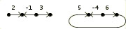 |
|---|
> Genome B

                        2 1 3 |

6 5 4 | | 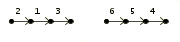 |
|---|
>Genome C

                        2 3 1 |

5 6 4 7 8 | | 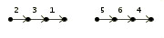 |
|---|
A simple example file can be found here.
A more complex example file that shows the possibilities can be
found here.
Optimal DCJ, rDCJ, HP, Inversion and Translocation Distance
and Sorting
The program can compute five different genomic distances and
optimal sorting scenarios: The DCJ, restricted DCJ, HP
(Hannenhalli & Pevzner), Inversion and Translocation distance
and an optimal corresponding sorting. All five distance and
sorting algorithms were implemented under the aspect of
efficiency and in most cases feature the most efficient
algorithms known until today. Links to the corresponding papers
can be found below.
Output example:
The output consists of the three tabs 'Genomes', 'Adjacencies'
and 'Graphics'.
The 'Genomes' tab either starts with informative messages, if a
genome comparison fails or singleton genes have to be removed
from a genome, or directly starts with the distance results as a
distance matrix, if the input consists of more than two genomes.
Otherwise the distances are returned in their context:
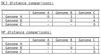
or if only Genome B and Genome C are compared with the HP
model:

A '-' in the distance results means that the distances for
this pair could not be calculated. Certain rules for the
different distance models, explained below under 'Rules', have to
be obeyed.
The graphical output will look like this for each pairwise
comparison:
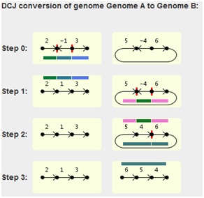
The fragments emerging from the two cuts (red vertical ticks
in the chromosome) of each step are highlighted by colored lines,
each with a different color. The lines for the current step are
located below the chromosome, while the lines depicting the
fragments of the previous step are located above the chromosome
of the current step.
Detailed explanations of the DCJ model and how it can be used
for calculating the rDCJ, HP, inversion and translocation
distances are given in the following papers:
- The DCJ model is explicated in [13] and improved and simplified in
[3].
- The restricted DCJ model is introduced in [9].
- How DCJ serves as a basis for HP, inversion and
translocation distances is explained in [4], while [5] provides the correct distance
formula. The running time of all distance computations is thus
linear.
The other models and the sorting algorithms are described
here:
- The HP model was first introduced in [6] and further studied in [10]. The sorting algorithm used in
this implementation is composed of: [12] as a basis for the
preprocessing including the correction provided by [8]. As suggested in [12] the sorting itself is then
carried out by the inversion sorting algorithm referred to in
the next item. Therefore, the sorting process runs in quadratic
time, which is determined by the used inversion sorting
algorithm.
- The inversion model was first solved in polynomial time in
[7] and the most efficient,
subquadratic sorting algorithm is described in [11]. Here, we implement the second
most efficient, quadratic time algorithm, also described in
[11], with the aid of the
data structures from [1].
- The translocation model and the implemented cubic sorting
algorithm are described in [2]. This algorithm was chosen
because in practice its running time is almost always
linear.
Rules
For a successful genome comparison the following rules have to
be obeyed:
- The DCJ distance calculation can handle all kinds of
genomes without restrictions
- The restricted DCJ model works for linear chromosomes and
directly reincoporates all emerging circular chromosomes in the
next step (modelling block interchanges and
transpositions).
- The HP distance calculation requires linear
chromosomes
- The translocation distance requires linear chromosomes with
the same telomeres.
- The inversion distance requires one linear chromosome with
the same telomeres in both genomes.
Program Usage - Step by Step
- First click on
 and choose at least one file that contains at
least two genomes. Or alternatively click
and choose at least one file that contains at
least two genomes. Or alternatively click  to work with a
small example file.
to work with a
small example file. - Then choose the genomes to compare in the lists below and
select one of the five possible scenarios.
 The 'All'
scenario means that all four scenarios are calculated at once,
if applicable.
The 'All'
scenario means that all four scenarios are calculated at once,
if applicable. - By pressing the
 Button the genomes will be compared. The results are
shown in the tabs in the lower part of the window.
Button the genomes will be compared. The results are
shown in the tabs in the lower part of the window. -
- The first tab
 first shows the distance in a matrix for more
than two genomes or otherwise in context with the chosen
scenario and afterwards the stepwise transformation for all
pairs of genomes.
first shows the distance in a matrix for more
than two genomes or otherwise in context with the chosen
scenario and afterwards the stepwise transformation for all
pairs of genomes. - The second tab
 shows the adjacencies (junctions) between
the genes. The suffix '_h' represents the head of a gene
and '_t' the tail of a gene. Chromosomes are separated by
'{content1} , {content2}' including the whitespaces for an
easier localization of a chromosome end.
shows the adjacencies (junctions) between
the genes. The suffix '_h' represents the head of a gene
and '_t' the tail of a gene. Chromosomes are separated by
'{content1} , {content2}' including the whitespaces for an
easier localization of a chromosome end. - The third tab
 contains a graphical representation of the
transformation of all pairs of genomes with highlighted
operations.
contains a graphical representation of the
transformation of all pairs of genomes with highlighted
operations.
- Before running the comparison:
-
- You can decide if only the distances are of interest
and the sorting scenarios are not needed (makes the
calculation also much faster). In this case deselect the
 checkbox, otherwise keep it selected.
 - You can choose a coloring method for the graphic:
If you select  each chromosome has a distinct
color, otherwise they have a white background.
each chromosome has a distinct
color, otherwise they have a white background.
- You can also adjust the size of the output using the size
slider with three different sizes.

- A graphic result can be saved as jpg image by clicking on
 .
. - The whole textual results can be saved in a txt file by
clicking on
 .
. - All values and results can be cleared by the
 button.
 - The
 button
terminates the program.
button
terminates the program. - If you want to look at the help directly from the program,
click on
 .
.
