|
The dominating source for RNA family models, and thus the most important use-case for Covarance Models (CMs), is
Rfam. And in fact, curators of Rfam and developers of
Infernal do closely cooperate. Infernal's CMs require all family member sequences to fold into one shared structure with only small deviations to gain good bit-scores. However, the grouping criteria of Rfam is different:
The ideal basis for a new family is an RNA element that has some known functional classification, is evolutionarily conserved, and has evidence for a secondary structure.
Rfam does not strictly insists on a single common structure. For example, take the tRNA family (RF00005, Rfam release 10.1). It is known that a minority of the tRNA structures form a stabilizing "variable stem-loop" in addition to the classical clover leaf structure. The
WikipediA article on tRNA, which Rfam uses to explain the family, does not fail to point to this fact. By a simple sequence length comparison, we found that 147 out of the 967 seed members constitute this minority. We also constructed a plausible consensus structure for this minority by aligning (
RNAforester) individual structure predictions from
tRNAscan-SE.
Replacing original SS
cons with our variable stem-loop enriched version cannot yield a different CM, because the majority of 820 members have gaps at the variable stem-loop positions and therefore model them as insertions, i. e. the introduced variable stem-loop sub-structure is taken out off SS
match. SS
match is SS
cons reduced by those alignment columns that have to many gaps. Informative covariance from base-pairs of this stem cannot be captured. On the other hand, enforcing SS
cons = SS
match by increasing allowed gap ratio, would impose large deletion costs on the 820 members, when aligning to the new model.
With the introduction of Ambivalent Covariance Models (aCM), we hope to open up a route to get over these shortcomings. Basically, an aCM is a CM constructed by multiple guide-trees, i. e. containing multiple consensus sequences SS
i
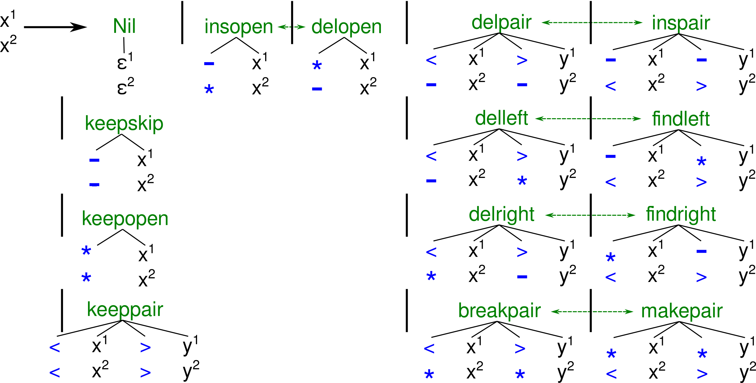
cons. These consensus structures should not be arbitrary structures, but be somehow compatible, i. e. can form one multiple alignment. This requires that all consensus structures have the same length, which can simply be achieved by introducing gaps. More thoughts have to be spend on defining what kinds of alignment columns should be allowed. For example, we think that the two consensus structures
(<<-*>**>, <<-*>-->) can explain a common evolution up to the point where two additional unpaired bases are inserted into the upper consensus. The double gaped column (-,-) should be allowed to enable inclusion of
rare sequences into M SA, which hold insertions relative to both consensus structures.
But we disallow alternative base-pair partners, like (<<**>>, <*<*>>) , since we cannot see a convincing evolutionary explanation. For example, base-pair slippage should better be
modeled via insertions. A formal definition of valid pairwise consensus structure alignments is given in the form of the ADP grammar G
ali_SS in the following Figure. Multiple consensus structures can be checked for compatibility by successively pairwise aligning them with G
ali_SS.
acmbuildTakes an RNA family, i.e. a multiple sequence alignment and one or more RNA consensus secondary structures, as input and constructs an ambivalent covariance model (aCM). An aCM is a stochastical search tool to quantify similarity of a single RNA sequence to an RNA family and is typically used to screen for homologs.
acmsearch
After you constructed an ambivalent covariance model with "acmbuild", you can use this stochastical search tool to analyse a set of RNA sequences for potential membership this family. Similarity is expressed in terms of bit-scores and for the best hit its alignment between RNA input and consensus structure is shown.
In-/Output values
INPUT :: BiBiServID
acmsearch needs an already build binary. You have to create such a binary by a run of acmbuild, which will return a BiBiServ ID. Use this ID to point this website to the correct binary!
INPUT :: RNA sequence(s)One or more ungapped RNA sequences.
INPUT :: RNA family
You must provide an RNA family, i.e. a multiple sequence alignment (MSA) and consensus structure(s) (SScons), in a Stockholm format. For details see the
Wikipedia article.
To support
ambivalent covariance models, you have to slightly extend the usual format and provide additional consensus structures. The normal feature name
SS_cons, must be prefixed with an identifying name, e.g. varLoop, and the delimiting character '
@'. Thus, a second "
#=GC varLoop@SS_cons" line should hold your second consensus structure.
To identify those MSA rows belonging to the varLoop consensus structure, their names have to be prefixed with the same label, e.g. a MSA row "AJ609482.1/1-130" should be named "varLoop@AJ609482.1/1-130".
OUTPUT :: acmbuild outputIn the case of success, the output is just the name of the compiled acmsearch binary and an example command line call for the generated binary. In other words, you should not care. Simply continue with an acmsearch functionality run!
OUTPUT :: acmsearch outputThe output format of an acmsearch run is loosely based on Infernals cmsearch output format. Detailed information can be found in their user guide. In short: The top line shows the predicted secondary structure of the model consensus sequence. Pairs are denoted by < and >, unpaired bases by * and insertions relative to the model with - characters. The second line shows the consensus sequence of the model. The highest scoring residue sequence is shown. Finally, the fourth line is the searched sequence.
Parameter
| Wbeta |
Wbeta is related to the "Query dependent banding (QDB)" accuracy heuristic [
NAW:EDD:2007]. In short, this is the accepted amount of probability mass one is willing to loose when restricting the yield size of a subtree in the Covariance Model to Wbeta, when applying QDB. This applies only to transition probabilities, emissions do not count. A larger Wbeta results in faster searches but also in decreased accuracy.
|
| eX |
The targeted amount of entropy when applying Expectation Maximization.
|
| ere |
This parameter influences the balancing between priors and posteriors when applying Expectation Maximization. Colloquially, it is the amount of wanted entropy in the system. It should not be smaller than 0.59.
|
| gapthresh |
We classify a column as a match-column, if its gap ratio is less than
gapthresh. The default value for this parameter is 0.5. The classification as an insert-column leads to the removal of the corresponding base in the consensus structure. If one column of a base-pair is classified as an insert-column, its partner must be transformed to an unpaired base in the consensus structure,
or removed as well, if its gap ratio is higher than
gapthresh.
|
| elself |
In principle, Covariance Models can also run in a local search mode. There, it must be possible to start and end at (almost) any state. When local ending at a state, there must be a further special EL state which consumes the remaining input bases via a self transition.
elself is this self transition probability.
Currently (26.3.2014), ACMs do not support a local search mode.
|
| iins |
Eddy et al. found that using emission probabilities for the insertion states of the Covariance Model disturbes performance. Thus, they suggest to use uniform probabilities for the symbols instead of the frequencies obtained by the training process.
However, with this parameter you can re-activate integration of trained emission probabilities.
|
| prior |
A Bayesian interpretation of probabilities composes them of Priors and Posteriors. Priors capture family independent knowledge, such as "thermophile bacteria show a higher GC content". This prior knowledge stems from experts and express what we know (or believe to know) about our system in general. Posteriors are gained via training, i.e. counting training sequences.
Should our training set be large enough, the influence of the priors will decrease and finally will loose their influence on the probabilities at all. This is called Ergodic Process. Due to this effect, it does not matter that some of the priors might be wrong.
Unfortunately, in practice the size of the training data is normally much to small to observe this Ergodic Process. Pseudocounts are an implementation of priors. Imagine an alignment column with some As, Cs and Gs but no Us. With posteriors only, it would never be possible to align an U to this column, even if all the remaining alignment would perfectly fit. Instead of completely prohibit an U, we want to assign a low probability with it. A sound stochastic model never sets probabilities to zero, but to a very low value at least. These values are the priors. The simplest way for priors, without the need of any prior knowledge, are pseudocounts. Before counting characters in the training data, we initialize each character occurrence with 1 instead of 0. Thus, the frequency in our example for U is 1(n+|A|) - where |A| is the size of the DNA alphabet - instead of 0. More advanced pseudocounts would use different initialization values e.g. for different characters.
We offers two sets of priors, namely "near zero priors" and "Dirichlet Mixtures for G5". The first set uses 10^-7 to initialize all values, the second set distinguishes between transition- and emission- probabilities. For the latter we uses Dirichlet mixtures.
|
| EM |
Expectation maximization should compensate for over-fitting, by finding a suitable trade-off between priors and posteriors.
In principle, Expectation Maximization is an alternative method for computing sequence weights for a MSA (=multiple sequence alignment), to avoid ignoring underrepresented sequence types. Another perspective is to see it as a method to avoid over-fitting for the maybe non representative set of known training data for a family. Expectation Maximization theory for Covariance Models is well presented in [
KRO:MIT:1995]. It"s practical implementation is described in [
JOH:2006].
|
| GSCweights |
Family sequences, i.e. MSA (= multiple sequence alignment) rows, do not contribute equally to the Covariance Model counts. Often the given RNA family, and thus the MSA, can be subdivided into, say, sub-families A and B. Due to different biological interests, different levels of experimental difficulties or whatever, the MSA might have many representatives for A, but only a few for B.
Since the Covariance Model should be able to detect both sub-families with equal strength, we can use different weights for training with the MSA sequences of both sub-families. The few sequences of B will have a higher weight than the many sequences of A, such that in the end both sub-family sequences will have the same influence to the final score.
With activated
GSCweights we use the "Gerstein /
Sonnhammer / Chothia tree weights", which is "unweighted pair group method using
arithmetic averages" (UPGMA) clustering (see pages 167ff. [
DUR:EDD:KRO:MIT:2002]) plus a method to infer
weights from the cluster tree [
GER:SON:CHO:1994].
|
|
|
